Triple Pendulum Motion Theory

Triple Pendulum Motion – Theory

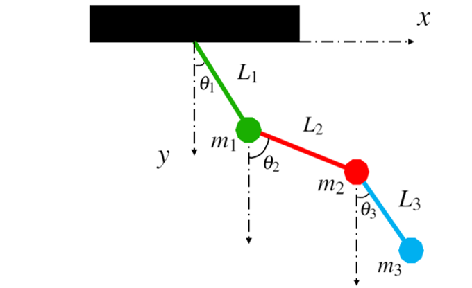
The diagram below represents the triple pendulum system—composed of three masses denoted as $m_1$ , $m_2$ , and $m_3$ —each connected by a rod of length $L_1$ , $L_2$ , and $L_3$ respectively. $\theta_1$ , $\theta_2$ , and $\theta_3$ are the angles between the the positive $y$ -axis and the respective rod, with clockwise rotation defined as being positive. Note that the coordinate system defines down as the positive $y$ -direction and right as the positive $x$ -direction. For this analysis we will assume the system is free of friction and that the mass of each rod is negligible (i.e., each rod is model as having a mass of zero).

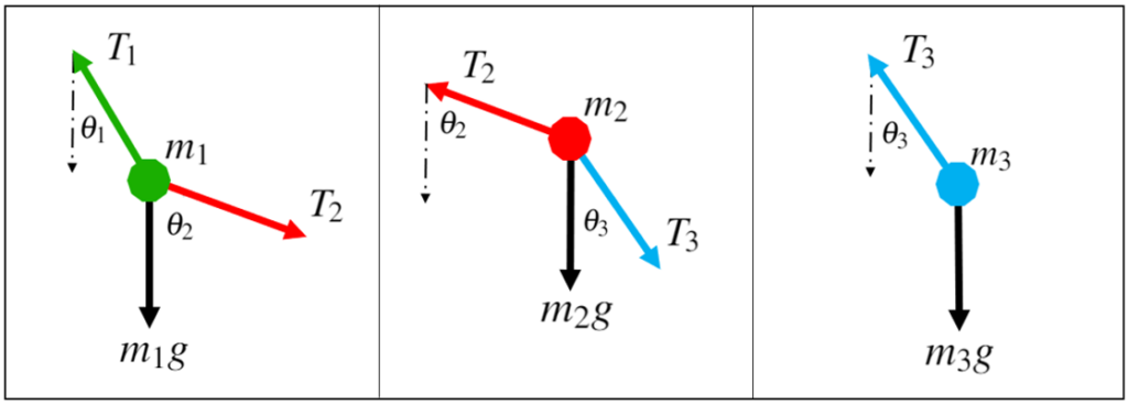
The position of each mass can be described in terms of three coordinate pairs, in other words, six variables (( $x_1, y_1$ ), ( $x_2, y_2$ ), & ( $x_3, y_3$ )). By relating $x_i$ and $y_i$ with $\theta_i$ the system’s position to be described in terms of three variables ( $\theta_1$ , $\theta_2$ , & $\theta_3$ ), thus, the system has three degrees of freedom, meaning we need three equations of motion. First, let us start with the masses free body diagram

Free Body Diagrams

Equations of Motion – Derivations

Newton’s Second Law:

(1) $\begin{equation*}\sum \boldsymbol{F} = m_i a_i = m_i ( \Ddot{x}_i \hat{i} + \Ddot{y}_i \hat{j} )\end{equation*}$

Applying Newton’s Second Law to the free body diagrams, we can get the six equations:

$m_1 \Ddot{x}_1 + T_1 \sin \theta_1 - T_2 \sin \theta_2 = 0$
$m_1 \Ddot{y}_1 + T_1 \cos \theta_1 - T_2 \cos \theta_2 - m_1g=0$
$m_2 \Ddot{x}_2 + T_2 \sin \theta_2 - T_3 \sin \theta_3 =0$
$m_2 \Ddot{y}_2 + T_2 \cos \theta_2 - T_3 \cos \theta_3 - m_2g=0$
$m_3 \Ddot{x}_3 + T_3 \sin \theta_3 =0$
$m_1 \Ddot{y}_3 + T_3 \cos \theta_3 - m_3g= 0$

Using these six equations, we can eliminate the tensile terms via substitution to obtain a system of three equations in term of $x_i$ , $y_i$ , and $\theta_i$ (and their time derivatives). These equations being:

(2) $\begin{equation*}g(m_1+m_2+m_3)\sin\theta_1-(m_1 \Ddot{y}_1+m_2\Ddot{y}_2+m_3\Ddot{y}_3)\sin \theta_1+(m_1\Ddot{x}_1+m_2\Ddot{x}_2+m_3\Ddot{x}_3)\cos\theta_1=0\end{equation*}$

(3) $\begin{equation*}g(m_2 + m_3)\sin \theta_2 - (m_2 \Ddot{y}_2 + m_3 \Ddot{y}_3)\sin \theta_2 + (m_2 \Ddot{x}_2 + m_3 \Ddot{x}_3)\cos \theta_2 = 0\end{equation*}$

(4) $\begin{equation*}m_3( g - \Ddot{y}_3) \sin \theta_3 + m_3 \Ddot{x}_3 \cos \theta_3 = 0\end{equation*}$

To express these equations only in terms of $\theta_i$ terms, we must determine expressions for the $x_i$ and $y_i$ terms, in terms of the $\theta_i$ . First let us express the position of the masses:

$x_1 &= L_1 \sin \theta_1$
$y_1 &= L_1 \cos \theta_1$
- $= L_1 \sin \theta_1 + L_2 \sin \theta_2$
- $= L_1 \cos \theta_1 + L_2 \cos \theta_2$
- $= L_1 \sin \theta_1 + L_2 \sin \theta_2 + L_3 \sin \theta_3$
- $= L_1 \cos \theta_1 + L_2 \cos \theta_2 + L_3 \cos \theta_3$

Now taking the first and second derivative of the position expressed in the general form (i.e., in terms of $x_i$ and $y_i$ ), we get:

$\Dot{x}_i &= L_i \Dot{\theta}_i \cos \theta_i$
$\Ddot{x}_i &= L_i \Ddot{\theta}_i \cos \theta_i - L_i \Dot{\theta}_i^2 \sin \theta_i$
$\Dot{y}_i &= -L_i \Dot{\theta}_i \sin \theta_i$
$\Ddot{y}_i &= -L_i \Ddot{\theta}_i \sin \theta_i - L_i \Dot{\theta}_i^2 \cos \theta_i$

Therefore,

$\Ddot{x}_1 &= L_1 \Ddot{\theta}_1 \cos \theta_1 - L_1 \Dot{\theta}_1^2 \sin \theta_1$
$\Ddot{y}_1 &= -L_1 \Ddot{\theta}_1 \sin \theta_1 - L_1 \Dot{\theta}_1^2 \cos \theta_1$
$\Ddot{x}_2 &= L_1 \Ddot{\theta}_1 \cos \theta_1 - L_1 \Dot{\theta}_1^2 \sin \theta_1 + L_2 \Ddot{\theta}_2 \cos \theta_2 - L_2 \Dot{\theta}_2^2 \sin \theta_2$
$\Ddot{y}_2 &= -L_1 \Ddot{\theta}_1 \sin \theta_1 - L_1 \Dot{\theta}_1^2 \cos \theta_1 - L_2 \Ddot{\theta}_2 \sin \theta_2 - L_2 \Dot{\theta}_2^2 \cos \theta_2$
$\Ddot{x}_3=L_1\Ddot{\theta}_1\cos\theta_1-L_1\Dot{\theta}_1^2\sin\theta_1+L_2\Ddot{\theta}_2\cos\theta_2-L_2\Dot{\theta}_2^2\sin\theta_2+L_3\Ddot{\theta}_3\cos\theta_3$ $-L_3\Dot{\theta}_3^2\sin\theta_3$
$\Ddot{y}_3 = -L_1 \Ddot{\theta}_1 \sin \theta_1 - L_1 \Dot{\theta}_1^2 \cos \theta_1 - L_2 \Ddot{\theta}_2 \sin \theta_2-L_2\Dot{\theta}_2^2 \cos\theta_2-L_3\Ddot{\theta}_3\sin\theta_3$ $-L_3\Dot{\theta}_3^2\cos\theta_3$

Now we are able to substitute all the $x_i$ and $y_i$ (and their time derivatives) into the three equations of motion. After substituting, rearranging, and simplifying, we finally get our three equations of motion:

(5) $\begin{equation*}$a_1\Ddot{\theta}_1 + a_2\Ddot{\theta}_2 + a_3\Ddot{\theta}_3 + a_4\dot{\theta}^2_1 + a_5\dot{\theta}_2^2 + a_6\dot{\theta}_3^2 + a_7 = 0$\end{equation*}$

where,
$a_1 &= (m_2 + m_3) L_1 \sin(\theta_1) \sin(\theta_2 - \theta_1) - m_1 L_1 \cos(\theta_2)$
$a_2 &= (m_2 + m_3) L_2 \sin(\theta_2) \sin(\theta_2 - \theta_1)$
$a_3 &= m_3 L_3 \sin(\theta_3) \sin(\theta_2 - \theta_1)$
$a_4 &= (m_2 + m_3) L_1 \cos(\theta_1) \sin(\theta_2 - \theta_1)$
$a_5 &= (m_2 + m_3) L_2 \cos(\theta_2) \sin(\theta_2 - \theta_1)$
$a_6 &= m_3 L_3 \cos(\theta_3) \sin(\theta_2 - \theta_1)$
$a_7 &= (m_2 + m_3)g \sin(\theta_2 - \theta_1) - m_1 g \sin(\theta_1) \cos(\theta_2)$

(6) $\begin{equation*}$b_1\Ddot{\theta}_1 + b_2\Ddot{\theta}_2 + b_3\Ddot{\theta}_3 + b_4\dot{\theta}^2_1 + b_5\dot{\theta}_2^2 + b_6\dot{\theta}_3^2 + b_7 = 0$\end{equation*}$

where,
$b_1 &= m_3 L_1 \sin(\theta_1) \sin(\theta_3 - \theta_2) - m_2 L_1 \cos(\theta_3) \cos(\theta_1 - \theta_2)$
$b_2 &= m_3 L_2 \sin(\theta_2) \sin(\theta_3 - \theta_2) - m_2 L_2 \cos(\theta_3)$
$b_3 &= m_3 L_3 \sin(\theta_3) \sin(\theta_3 - \theta_2)$
$b_4 &= m_3 L_1 \cos(\theta_1) \sin(\theta_3 - \theta_2) + m_2 L_1 \cos(\theta_3) \sin(\theta_1 - \theta_2)$
$b_5 &= m_3 L_2 \cos(\theta_2) \sin(\theta_3 - \theta_2)$
$b_6 &= m_3 L_3 \cos(\theta_3) \sin(\theta_3 - \theta_2)$
$b_7 &= -(m_2 + m_3)g \sin(\theta_2)\cos(\theta_3) + m_3 g \cos(\theta_2) \sin(\theta_3)$

(7) $\begin{equation*}$c_1\Ddot{\theta}_1 + c_2\Ddot{\theta}_2 + c_3\Ddot{\theta}_3 + c_4\dot{\theta}^2_1 + c_5\dot{\theta}_2^2 + c_6 = 0$\end{equation*}$

where,
$c_1 &= L_1 \cos(\theta_1 - \theta_3)$
$c_2 &= L_2 \cos(\theta_2 - \theta_3)$
$c_3 &= L_3$
$c_4 &= L_1 \sin(\theta_3 - \theta_1)$
$c_5 &= L_2 \sin(\theta_3 - \theta_2)$
$c_6 &= g \sin(\theta_3)$

We have a system of second order, ordinary differential equations (ODEs). In order to solve the system of equations numerically using MATLAB, it must be transformed into a system of six coupled first order ODEs. To do this, I will define the vector $\boldsymbol{z}$ as:

(8) $\begin{equation*}\boldsymbol{z} =\begin{bmatrix}z_1 = \theta_1 \\z_2 = \dot{\theta_1} \\z_3 = \theta_2 \\z_4 = \dot{\theta_2} \\z_5 = \theta_3 \\z_6 = \dot{\theta_3} \\\end{bmatrix}\end{equation*}$

therefore, the time derivative of $z$ would give:

(9) $\begin{equation*}\boldsymbol{\dot{z}} =\begin{bmatrix}\dot{z_1} \\\dot{z_2} \\\dot{z_3} \\\dot{z_4} \\\dot{z_5} \\\dot{z_6} \\\end{bmatrix} = \begin{bmatrix}z_2 = \dot{\theta_1} \\\dot{z_2} = \Ddot{\theta_1} \\z_4 = \dot{\theta_2} \\\dot{z_4} = \Ddot{\theta_2} \\z_6 = \dot{\theta_3} \\\dot{z_6} = \Ddot{\theta_3} \\\end{bmatrix}\end{equation*}$

By writing the EOM—equations (5), (6), and (7)—in terms of $\boldsymbol{z}$ , the equations of motion can now be expressed in as a system of six coupled first order ODEs, in other words, the system of equations only contains $z_i$ and $\dot{x}_i$ terms. The resulting equations are:

(10) $\begin{equation*}a_1\dot{z}_2 + a_2\dot{z}_4 + a_3\dot{z}_6 + a_4 z^2_2 + a_5 z^2_4 + a_6 z^2_6 + a_7 = 0\end{equation*}$

(11) $\begin{equation*}b_1\dot{z}_2 + b_2\dot{z}_4 + b_3\dot{z}_6 + b_4 z^2_2 + b_5 z^2_4 + b_6 z^2_6 + b_7 = 0\end{equation*}$

(12) $\begin{equation*}c_1\dot{z}_2 + c_2\dot{z}_4 + c_3\dot{z}_6 + c_4 z^2_2 + c_5 z^2_4 + c_6 = 0\end{equation*}$

(13) $\begin{equation*}z_2 &= \dot{z}_1\end{equation*}$

(14) $\begin{equation*}z_4 &= \dot{z}_3\end{equation*}$

(15) $\begin{equation*}z_6 &= \dot{z}_5\end{equation*}$

Equations (10), (11), and (12) can be expressed in matrix form as:

(16) $\begin{equation*}\hspace{10mm} \begin{bmatrix}a_1 && a_2 && a_3 \\b_1 && b_2 && b_3 \\c_1 && c_2 && c_3\end{bmatrix} \begin{bmatrix}\dot{z}_2 \\\dot{z}_4 \\\dot{z}_6\end{bmatrix} = \begin{bmatrix}-(a_4 z^2_2 + a_5 z^2_4 + a_6 z^2_6 + a_7) \\-(b_4 z^2_2 + b_5 z^2_4 + b_6 z^2_6 + b_7) \\-(c_4 z^2_2 + c_5 z^2_4 + c_6)\end{bmatrix}&&\end{equation*}$

Such a system of equations can easily be numerically solved using back division in MATLAB, where if we let,

(17) $\begin{equation*}\hspace{10mm}\begin{bmatrix}M\end{bmatrix} = \begin{bmatrix}a_1 && a_2 && a_3 \\b_1 && b_2 && b_3 \\c_1 && c_2 && c_3\end{bmatrix} and \begin{bmatrix}N\end{bmatrix} = \begin{bmatrix}-(a_4 z^2_2 + a_5 z^2_4 + a_6 z^2_6 + a_7) \\-(b_4 z^2_2 + b_5 z^2_4 + b_6 z^2_6 + b_7) \\-(c_4 z^2_2 + c_5 z^2_4 + c_6)\end{bmatrix}&&\end{equation*}$

Then we can solve by:

(18) $\begin{flalign*}\hspace{10mm} \begin{bmatrix}\dot{z}_2 \\\dot{z}_4 \\\dot{z}_6\end{bmatrix} = \begin{bmatrix}M\end{bmatrix} \backslash \begin{bmatrix}N\end{bmatrix}&&\end{flalign*}$

Now, $\dot{z}_2$ , $\dot{z}_4$ , and $\dot{z}_6$ can be solved in terms of $z_2$ , $z_4$ , $z_6$ , and constants by solving the system of equations: (10), (11), and (12). This was done in MATLAB by first writing equations (10), (11), and (12) as:

Solving the Equations of Motion via MATLAB – Establishing the Structure

Video tutorials coming soon!